Geodesic Momentum Sampling for Masked Discrete Diffusion Language Models

📄 Read the Full Paper (PDF)

Abstract

Masked discrete diffusion language models generate text through a sequence of categorical denoising transitions. We study an inference-time modification that treats each per-token categorical prediction as a point on the Fisher--Rao statistical manifold. The square-root map embeds the categorical simplex into the positive orthant of a hypersphere, where closed-form spherical interpolation is available. At each reverse step, we recursively continue the great-circle arc from the previous extrapolated prediction through the current model prediction, map the result back to a categorical distribution, and insert it into the original MDLM or SEDD transition. We call the method geodesic momentum sampling.

We give a precise geometric derivation, prove equivalence between the unprojected update and an exponential-map continuation, and show that its small-angle coefficients coincide with the coefficients of variable-step Adams--Bashforth two-step extrapolation. We also delimit this analogy: the method extrapolates prediction distributions rather than tangent vector fields, retains stochastic categorical jumps, and uses a positive-orthant projection. It is therefore not a second-order probability-flow ODE solver, and no second-order convergence claim is made. Archived experiments on OpenWebText checkpoints suggest improved GPT-2 generative perplexity for MDLM at 10--100 reverse steps and for SEDD at 10--50 steps.

Introduction

Discrete diffusion language models offer parallel, bidirectional generation, but accurate sampling often requires many reverse transitions. MDLM simplifies absorbing-state diffusion through a substitution parameterization and provides an cached sampler. SEDD instead learns concrete score ratios and admits an analytic reverse transition. Both models nevertheless operate by repeatedly producing categorical distributions over a vocabulary.

Information geometry supplies a natural geometry for these distributions. The interior of the categorical simplex carries the Fisher--Rao metric; the square-root map identifies it, up to a constant scale, with the positive orthant of a sphere. This construction underlies Fisher-Flow and the continuous Riemannian diffusion language model (RDLM). Those methods learn or simulate continuous flows on the sphere. Our setting is different: we preserve pretrained discrete MDLM and SEDD models and modify only their inference-time categorical predictions.

The main contributions are:

• We formulate recursive geodesic extrapolation of categorical predictions using the exact square-root embedding and spherical linear interpolation (SLERP).
• We show that the unprojected update is an exponential-map continuation and derive its local Adams--Bashforth-like coefficient structure.
• We instantiate the same geometric operator at two different interfaces: the clean-token prediction in MDLM and the analytic transition distribution in SEDD.
• We state invariants and the precise limits of the high-order analogy. In particular, we do not identify the algorithm with an RDLM probability-flow ODE solver.
• We report MDLM and SEDD quality results across six reverse-step counts.

Background

Categorical Fisher--Rao geometry

Let

$$\Delta^{V-1} = \left\{p\in\mathbb{R}^{V}: p_k\ge 0,\ \sum_{k=1}^{V}p_k=1\right\}$$

be the categorical probability simplex. On its interior, a tangent vector satisfies $\sum_k v_k=0$, and the Fisher--Rao metric is

$$g_p(v,w)=\sum_{k=1}^{V}\frac{v_kw_k}{p_k}.$$

Proposition 1 (Square-root isometry) Define $\Psi:\operatorname{int}(\Delta^{V-1})\rightarrow\mathbb{S}^{V-1}_+(2)$ by $\Psi(p)=2\sqrt{p}$ elementwise, where $\mathbb{S}^{V-1}_+(2)$ is the positive orthant of the sphere of radius two. Then $\Psi$ is an isometry between the Fisher--Rao metric and the metric induced by the ambient Euclidean space.

Proof. For $\psi_k=2\sqrt{p_k}$, we have $d\psi_k=dp_k/\sqrt{p_k}$. Therefore

$$\lVert d\psi\rVert_2^2 =\sum_k\frac{dp_k^2}{p_k} =ds_{\mathrm{FR}}^2.$$

Moreover, $\lVert\psi\rVert_2^2=4\sum_k p_k=4$, so $\psi$ lies on the radius-two sphere.

The implementation uses the unit-sphere coordinate

$$u(p)=\sqrt{p}\in\mathbb{S}^{V-1}_+,$$

which differs only by the constant factor two. For $p,q\in\operatorname{int}(\Delta^{V-1})$, their spherical angle is

$$\omega(p,q) =\arccos\langle u(p),u(q)\rangle =\arccos\left(\sum_k\sqrt{p_kq_k}\right),$$

and the Fisher--Rao distance under the radius-two convention is $d_{\mathrm{FR}}(p,q)=2\omega(p,q)$. This formula extends continuously to the closed simplex and yields its metric completion; boundary points themselves are not smooth points of the Fisher--Rao Riemannian manifold.

Masked discrete diffusion and MDLM

Let $\mathtt{m}$ denote an absorbing mask state and let $\sigma(t)$ be the integrated noise schedule. The probability of having moved to the mask by time $t$ is

$$m(t)=1-\exp[-\sigma(t)].$$

For a reverse step $t>s$, MDLM predicts a clean-token distribution $p_{\theta,t}(\cdot\mid x_t)$ whose absorbing-state parameterization satisfies $p_{\theta,t}(\mathtt{m}\mid x_t)=0$ and $\sum_{k\ne\mathtt{m}}p_{\theta,t}(k\mid x_t)=1$. When $x_t=\mathtt{m}$, the baseline implementation samples from the unnormalized weights

$$\widetilde q^{\mathrm{MDLM}}_{s\mid t}(k\mid x_t=\mathtt{m})= \begin{cases} [m(t)-m(s)]p_{\theta,t}(k\mid x_t), & k\neq\mathtt{m},\\ m(s), & k=\mathtt{m}. \end{cases}$$

Their common normalization is immaterial for categorical sampling. When $x_t\neq\mathtt{m}$, the absorbing reverse sampler copies the already unmasked token. The cached sampler reuses $p_{\theta,t}$ until the discrete state changes.

SEDD analytic transitions

SEDD learns a concrete score ratio that approximates $p_t(y)/p_t(x)$. Let $r_\theta(x_t,t)$ denote the learned score vector, let $\mathcal{S}_{\Delta\sigma}$ denote the staggered-score transform, and let $K_{\Delta\sigma}(x_t,\cdot)$ denote the transported forward kernel. The analytic sampler uses

$$\widetilde q^{\mathrm{SEDD}}_{s\mid t} =\mathcal{S}_{\Delta\sigma}\!\left(r_\theta(x_t,t)\right) \odot K_{\Delta\sigma}(x_t,\cdot), \qquad \Delta\sigma=\sigma(t)-\sigma(s),$$

followed by categorical sampling. Our SEDD variant applies geometry to the normalized version of this transition, not to the score vector itself.

Geodesic Momentum Sampling

A common distribution interface

For each batch element and sequence position, define a categorical distribution $z_i\in\Delta^{V-1}$ at reverse index $i$:

$$z_i = \begin{cases} p_{\theta,t_i}(\cdot\mid x_{t_i}), & \text{MDLM},\\ \operatorname{Normalize}(\widetilde q^{\mathrm{SEDD}}_{t_{i+1}\mid t_i}), & \text{SEDD}. \end{cases}$$

The raw spherical coordinate is $u_i=\sqrt{z_i}$. Let $\widehat u_{i-1}$ be the previous extrapolated coordinate. This recursive choice is important: the method has persistent momentum rather than retaining only two raw predictions.

Exact spherical continuation

For unit vectors $a,b\in\mathbb{S}^{V-1}$ with angle $\omega=\arccos\langle a,b\rangle\in(0,\pi)$, SLERP is

$$\operatorname{Slerp}(a,b;\tau) =\frac{\sin[(1-\tau)\omega]}{\sin\omega}a +\frac{\sin(\tau\omega)}{\sin\omega}b.$$

Interpolation uses $\tau\in[0,1]$. We instead choose $\tau=1+\alpha_i$:

$$e_i =\frac{\sin(-\alpha_i\omega_i)}{\sin\omega_i}\widehat u_{i-1} +\frac{\sin[(1+\alpha_i)\omega_i]}{\sin\omega_i}u_i, \quad \omega_i=\arccos\langle\widehat u_{i-1},u_i\rangle.$$

Proposition 2 (Exponential-map representation) For distinct, non-antipodal $a,b\in\mathbb{S}^{V-1}$ and $\alpha\ge 0$,

$$\operatorname{Slerp}(a,b;1+\alpha) =\operatorname{Exp}_b\!\left[-\alpha\operatorname{Log}_b(a)\right].$$

Thus the equation exactly continues the great-circle arc from $a$ through $b$ by an additional fraction $\alpha$ before the positivity operation described below.

Proof. The curve $\gamma(\tau)=\operatorname{Slerp}(a,b;\tau)$ is the unique shortest great-circle segment from $a$ to $b$ for $\tau\in[0,1]$. At $b=\gamma(1)$, $-\operatorname{Log}_b(a)$ is the forward continuation tangent with norm $\omega$. Applying $\operatorname{Exp}_b$ to the scaled vector $-\alpha\operatorname{Log}_b(a)$ advances by arc length $\alpha\omega$, which is exactly $\gamma(1+\alpha)$.

At $a=b$ (equivalently, $\omega=0$), we define $\operatorname{Slerp}(a,a;\tau)=a$ by continuous extension, and the proposition remains valid.

Positive-orthant projection and probability recovery

Great-circle extrapolation may leave the positive orthant. The archived implementation uses

$$\operatorname{Proj}_{+}(e)=\frac{[e]_+}{\lVert[e]_+\rVert_2}, \qquad [e]_{+,k}=\max(e_k,0),$$

and recovers

$$\widehat z_{i,k}=(\widehat u_{i,k})^2, \qquad \widehat u_i=\operatorname{Proj}_{+}(e_i).$$

Proposition 3 (Probability validity) Whenever $\lVert[e_i]_+\rVert_2>0$, the recovered vector $\widehat z_i$ lies in $\Delta^{V-1}$.

Proof. Each component is a square and is therefore nonnegative. Since $\widehat u_i$ has unit norm, $\sum_k\widehat z_{i,k}=\sum_k\widehat u_{i,k}^2=1$.

This projection is a practical domain correction, not part of the exact Fisher--Rao geodesic.

Step coefficient and the AB2 analogy

Let the descending reverse grid be $t_0>t_1>\cdots>t_N$ and define positive step magnitudes $h_i=t_i-t_{i+1}$. The implementation uses

$$\alpha_i=c_i\frac{h_i}{2h_{i-1}},\qquad \alpha_0=0.$$

For SEDD, the archived runs use $c_i=1$. For MDLM,

$$c_i=c\min\left(1,\frac{h_i}{h_{\mathrm{ref}}}\right), \qquad c=1,\quad h_{\mathrm{ref}}=\frac{1}{50}.$$

Proposition 4 (Local linear form) For fixed $\alpha$ and $\omega=\arccos\langle a,b\rangle\rightarrow0$,

$$\operatorname{Slerp}(a,b;1+\alpha) =(1+\alpha)b-\alpha a+O(\omega^2).$$

With $c_i=1$ and $r_i=h_i/h_{i-1}$, the leading coefficients are $(1+r_i/2,-r_i/2)$, matching the coefficients of variable-step AB2.

Proof. Using $\sin(\beta\omega)/\sin\omega=\beta+O(\omega^2)$ gives $\sin(-\alpha\omega)/\sin\omega=-\alpha+O(\omega^2)$ and $\sin[(1+\alpha)\omega]/\sin\omega=1+\alpha+O(\omega^2)$.

Instantiation for MDLM and SEDD

For MDLM, $\widehat z_i$ replaces $p_{\theta,t_i}$; already unmasked tokens remain fixed. For SEDD, $\widehat z_i$ directly replaces the normalized analytic transition. In both cases, the next token state is sampled with Gumbel-max. The algorithm therefore keeps all neural-network inputs discrete.

Theoretical Scope and Non-Claims

The method preserves several exact properties:

1. Discrete-state compatibility. The model always receives integer token indices.
2. First-step equivalence. Since $\alpha_0=0$, the first categorical transition equals the corresponding baseline transition under the same random draw.
3. Simplex validity. Subject to the nonzero projection condition, every extrapolated distribution is nonnegative and normalized.
4. MDLM absorbing structure. Tokens already unmasked remain fixed, exactly as in the uncached MDLM reverse transition.

However, the sampled sequence $x_{t_i}$ changes stochastically, so the sequence $z_i$ is a collection of conditional predictions along a random path, not a deterministic marginal curve $p_t$. We therefore make no claim of marginal preservation, local truncation error $O(h^3)$, or global convergence $O(h^2)$.

Experimental Evaluation

The scripts compare MDLM against its ddpm_cache sampler and SEDD against its analytic sampler. Both use OpenWebText checkpoints and sequence length 1024. The reverse-step counts are 10, 20, 50, 100, 256, and 512. The quality metrics are:

• token-weighted perplexity under GPT-2, where lower is better; and
• Jensen--Shannon divergence between generated and reference unigram token histograms, where lower is better.

Quality results

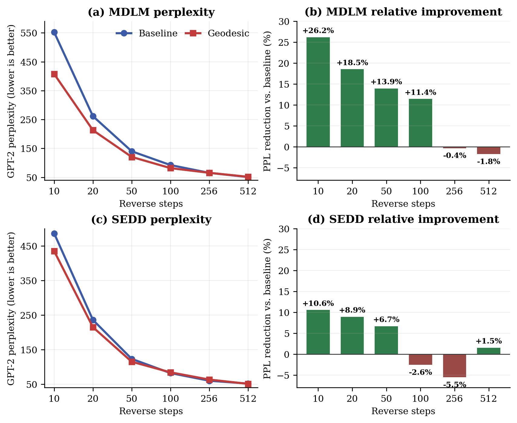Figure 1: Perplexity results. Left panels show raw GPT-2 perplexity. Right panels show the relative PPL reduction, so positive bars indicate improvement.

At 10, 20, 50, and 100 MDLM steps, the geodesic samples have respectively 26.18%, 18.53%, 13.95%, and 11.42% lower GPT-2 perplexity. At 256 and 512 steps, the difference vanishes and slightly favors the baseline. This pattern is consistent with the method's intended use as a low-step correction.

SEDD shows smaller perplexity reductions at 10--50 steps, degradation at 100--256, and a small improvement at 512.

Conclusion

We presented geodesic momentum sampling, an inference-time modification for MDLM and SEDD that recursively extrapolates categorical predictions on the Fisher--Rao square-root sphere. The update has an exact exponential-map interpretation before positive-orthant projection, and its local coefficients match variable-step AB2 coefficients. The algorithm nevertheless operates on prediction points along a stochastic discrete path, not on parallel-transported vector fields of a probability-flow ODE. Its mathematically accurate characterization is therefore recursive Fisher--Rao spherical extrapolation, not a proven second-order Riemannian solver.